Microarray Statistics

top
	sample output: Click Here to view a typical tab delimited output imported into excel from the microarray normalization package M.A.N..
top
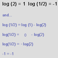
	Why do we log the normalized ratios? We are interested in genes of 2-fold interest.
top
	Now lets take a look at the logged values of 0.5 and 2.0:
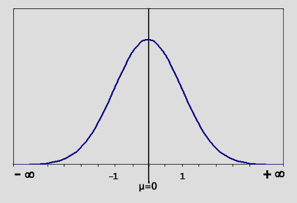
	Now examine the graph in (fig.2).
	(fig. 2)
top
	We use a 2-sample Student's T-test (fig. 3) on the logged values by setting "mu" to zero. This measures the difference between a sample mean and zero. The t-test result is used to obtain your p-value (see fig. 4).
	(fig. 3)
	(note - "S" = "sample" standard deviation, not a population standard deviation: (n-1) versus (n) degrees of freedom respectively.
top
	The following is the p-value formula and uses the result from the above t-test (note the " t "). The p-value will represent an area (fig. 5) under the probability curve (integral) which will be less than or greater than the significance level. The significance level is defined by the user as alpha (normally .05).
	(fig. 4)
top
	(fig. 5)
	We will reject the NULL hypothesis (H0) if the p-value is less than the significance level of alpha (normally .05).
	(fig. 6)
	This means we will keep those genes with significant p-values.
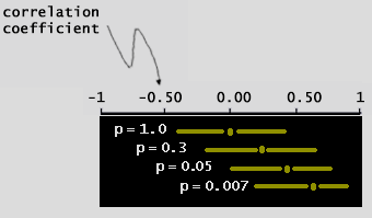
	In this system "significant" p-values reflect the probability that a specific gene is up- or down-regulated and gives an estimate of the quality of the technical replicates. Therefore one may discount a number of genes due to poor replication or dye-biases. Academically speaking, a low p-value for the statistical test points to rejection of the null hypothesis because it indicates how unlikely it is that a test statistic as extreme, or more extreme (positive or negative), than the one given by this data will be observed if the null hypothesis is true. What is considered a low, or significant p-value?. Normally alpha is set to 0.05 and any p-values below that mark are considered "significant". p-values do not simply provide a "yes" or "no" answer. They provide a sense of the strength of evidence against the null hypothesis. Additionally a p-value <= 0.05 produces a complimentary "Confidence Interval" of 95 % that does not cross zero (0) (note the position of "mu" in the confidence interval formula below):
	(fig. 7)
	(fig. 9) shows the relationship between a p-value <= 0.05 and it's complimentary 95% confidence interval that does not cross zero (0):
	(fig. 8)
top
	If your confidence interval includes 0 and you have a significant p-value, then a Type I error (false positive), or a Type II error (false negative), result may exist. Here you would want to consider a Bonferonni adjustment.
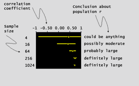
	Small confidence intervals that do not include zero give support to the validity of your p-values. Running a larger group of samples will decrease the size of the confidence interval and decrease the possibility of including zero. Lets see how this works in (fig. 9):
	(fig. 9)
top
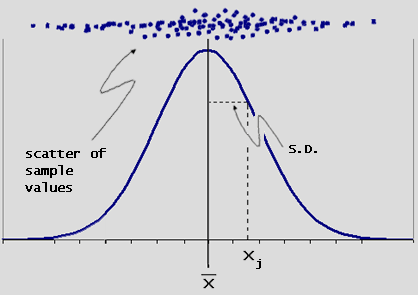
	Great, now we know all about p-values and their relative confidence intervals. So what about Standard Deviation. and Variance. Well Standard Deviation (fig. 11) numerically speaking is the square root of variance:
	(fig. 11)
	And Variance (fig. 12) is the mean value of all the differences from the mean multiplied by themselves (squared).
	(fig. 12) sample variance
top
	So we can define Standard Deviation as a measure of the distribution spread. Simply put: take the distance of each number from the mean, square it, average the result, then take the square root. In short, it's the root mean square of the distances (or differences) from the mean. (Usually abbreviated as SD in scientific journals and as S in stats books and stats journals.)
	(fig. 13)
top
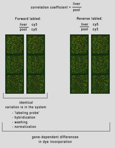
	But what sources of variation can we have in our microarray experiment? 1 - spot deposition on slide. 2 - blocking 3 - labeling probe 4 - hybridization 5 - washing 6 - scanning 7 - normalization 8 - gene specific differences in dye incorporation. In (fig. 14) we have a Correlation Coefficient between a liver sample and a pooled liver control. By examining the forward (or reversed) slides we can see variation in the system, such as hybridization, washing, etc. Examining the forward slides with the reversed slides can reveal gene-dependent dye incorporation.
	What's a Correlation Coefficient ?
	(fig. 14)
top
	Great! I've got variance, so what. Well let's return to our sample data from above and work with all these neat numbers. 1 - Sort data by the p-value. 2 - Collect all genes with p-values <= alpha (.05 - remember the area under the curve..... p-value?) 3 - Calculate the non-logged average per gene (see column T in normalized output ).
	Examine the normalized output for gene number 8797, the "mouse-ig h-chain gene". (highlighted in yellow) and notice the following points: 1 - The p-value is less than our alpha = 0.05 - meaning the gene is significant. 2- The confidence interval does not contain 0 - meaning we don't have TypeI/II errors. 3 - The variance = .032 = (0.18)^2 = (S.D.)^2 4 - The non-logged average is 1.615, indicating that this genes expression is 161.5% (+- 0.032 of variance), or up-regulated.
	NOTE: - you will get stronger p-values and confidence intervals when the number of samples (slides) you normalize is > 10. NOTE - precision of the statistical model above relies upon: 1 - Independence of Observations: independence of observations refers to the notion that the value of one datum is unrelated to any other datum. In other words, knowing the value of one observation gives you no information about the value of any other. 2 - Normality of sampling distribution: The sampling distribution of any outcome statistic is the distribution you would expect to get for the values of the statistic, if you repeated your study many times.
top